●해당 데이터 세트는 불균형 데이터 세트로, 레이블인 Class 속성은 매우 불균형한 분포를 가짐
Class 0 → 정상적인 신용카드 트랜잭션 데이터
Class 1 → 신용카드 사기 트랜잭션
●전체 데이터의 약 0.172%만이 레이블 값이 1, 즉 사기 트랜잭션임
●일반적으로 사기 검출, 이상 검출과 같은 데이터 세트는 이처럼 레이블 값이 극도로 불균형한 분포를 가지기 쉬움. 왜냐하면 사기와 같은 이상 현상은 전체 데이터에서 차지하는 비중이 매우 적을 수밖에 없기 때문
1. Data load
●필요한 모듈 및 패키지 불러오기
import pandas as pd
import numpy as np
import matplotlib.pyplot as plt
import warnings
warnings.filterwarnings('ignore')
%matplotlib inline
●데이터 불러오기
card_df = pd.read_csv(r'C:\Users\82102\PerfectGuide\4장\creditcard.csv')
card_df.head()
card_df.info()
card_df.isnull().sum()
card_df.describe()
●데이터 불균형 확인
card_df['Class'].value_counts()
- Time 피처의 경우 데이터 생성 관련한 작업용 속성으로서 큰 의미가 없기에 제거
- Amount 피처는 신용카드 트랜잭션 금액
- Class는 레이블로서 0의 경우 정상, 1의 경우 사기 트랜잭션
- 결측값은 없음
- Class는 int형, 나머지 피처들은 float형
2. 데이터 1차 가공 및 모델 학습/예측/평가
●Time 피처 삭제
# 인자로 입력받은 DataFrame을 복사한 뒤 Time 피처만 삭제하고 복사된 DataFrame 반환하는 함수 생성
def get_preprocessed_df(df=None):
    df_copy = df.copy()
    df_copy.drop('Time', axis=1, inplace=True)
    return df_copy
●학습 / 테스트 데이터 세트 분리
- stratify 방식 사용: 불균형 데이터 세트이므로 학습 / 테스트 데이터 세트는 원본 데이터와 같은 레이블 값 분포로 맞춰주고 → 학습 / 테스트 데이터 세트의 레이블 값 분포를 동일하게 설정
from sklearn.model_selection import train_test_split

# 사전 데이터 가공 후 학습과 테스트 데이터 세트를 반환하는 함수 생성
def get_train_test_dataset(df=None):
    # Time 피처를 삭제한 df를 받아옴
    df_copy = get_preprocessed_df(df)

    # 피처, 레이블 분리
    X_features = df_copy.iloc[:, :-1]
    y_target = df_copy.iloc[:, -1]

    # 학습 데이터 세트, 테스트 데이터 세트 분리
    X_train, X_test, y_train, y_test = train_test_split(X_features, y_target, test_size=0.3, random_state=0, stratify=y_target)

    return X_train, X_test, y_train, y_test
●원본 데이터 함수 적용
X_train, X_test, y_train, y_test = get_train_test_dataset(card_df)- 학습 데이터 세트와 테스트 데이터 세트의 레이블 값 비율이 서로 비슷하게 분할됐는지 확인
print('학습 데이터 레이블 값 비율')
print(y_train.value_counts() / y_train.shape[0] * 100)
print('\n')
print('테스트 데이터 레이블 값 비율')
print(y_test.value_counts() / y_test.shape[0] * 100)
●모델 성능 평가 함수 선언
from sklearn.metrics import *

def get_clf_eval(y_test, pred=None, pred_proba=None):
    confusion = confusion_matrix(y_test, pred)
    accuracy = accuracy_score(y_test, pred)
    precision = precision_score(y_test, pred)
    recall = recall_score(y_test, pred)
    f1 = f1_score(y_test, pred)
    roc_auc = roc_auc_score(y_test, pred_proba)

    print('오차 행렬')
    print(confusion)
    print('정확도:{0:.4f}, 정밀도:{1:.4f}, 재현율:{2:.4f}, F1:{3:.4f}, AUC:{4:.4f}'.format(accuracy, precision, recall, f1, roc_auc))
●모델 학습/예측/평가
1) LogisticRegression
from sklearn.linear_model import LogisticRegression

lr_clf = LogisticRegression(max_iter=1000)
lr_clf.fit(X_train, y_train)
lr_pred = lr_clf.predict(X_test)
lr_pred_proba = lr_clf.predict_proba(X_test)[:, 1]

get_clf_eval(y_test, lr_pred, lr_pred_proba)
- 매번, 모델 학습/예측/평가 하는 코드 작성이 귀찮으므로 반복적으로 모델을 변경해 학습/예측/평가 하는 함수 생성
def get_model_train_eval(model, ftr_train=None, ftr_test=None, tgt_train=None, tgt_test=None):
    model.fit(ftr_train, tgt_train)
    pred = model.predict(ftr_test)
    pred_proba = model.predict_proba(ftr_test)[:, 1]

    get_clf_eval(tgt_test, pred, pred_proba)
2) LightGBM
LightGBM 2.1.0 이상의 버전에서 boost_from_average 파라미터의 default가 False에서 True로 변경됨. 레이블 값이 극도로 불균형한 분포를 이루는 경우 boost_from_average=True 설정은 재현율 및 ROC-AUC 성능을 매우 크게 저하시킴. 따라서 레이블 값이 극도로 불균형할 경우 boost_from_average를 False로 설정하는 것이 유리
# 본 데이터 세트는 극도로 불균형한 레이블 값 분포도를 가지므로 boost_from_average=False로 설정
from lightgbm import LGBMClassifier

lgbm_clf = LGBMClassifier(n_estimators=1000, num_leaves=64, n_jobs=-1, boost_from_average=False)

get_model_train_eval(lgbm_clf, ftr_train=X_train, ftr_test=X_test, tgt_train=y_train, tgt_test=y_test)
3. 데이터 분포도 변환 후 모델 학습/예측/평가
왜곡된 분포도를 가지는 데이터를 재가공한 뒤에 모델을 다시 테스트 해보자
●Amount 피처 분포도 확인
Amount 피처는 신용 카드 사용 금액으로 정상/사기 트랜잭션을 결정하는 매우 중요한 피처일 가능성이 높다.
import seaborn as sns

plt.figure(figsize=(8,4))
plt.xticks(range(0, 30000, 1000), rotation=60)
sns.histplot(card_df['Amount'], bins=100, kde=True)
plt.show()
Amount 피처는 1000 이하인 데이터가 대부분이며, 26000까지 드물지만 많은 금액을 사용한 경우가 발생하면서 꼬리가 긴 형태의 분포 곡선을 가진다
대부분의 선형 모델은 중요 피처들의 값이 정규분포 형태를 유지하는 것을 선호하기 때문에 Amount 피처를 표준 정규분포 형태로 변환하자
●standardscaler를 이용해 Amount 피처 변환
from sklearn.preprocessing import StandardScaler

def get_preprocessed_df(df=None):
    df_copy = df.copy()

    # Amount 피처를 표준 정규분포 형태로 변환
    scaler = StandardScaler()
    amount_n = scaler.fit_transform(df_copy['Amount'].values.reshape(-1,1))

    # 변환된 Amount 피처를 Amount_Scaled로 피처명 변경후 DataFrame 맨 앞 컬럼으로 추가
    df_copy.insert(0, 'Amount_Scaled', amount_n)

    # 기존 Time, Amount 피처 삭제
    df_copy.drop(['Time', 'Amount'], axis=1, inplace=True)

    return df_copy
●모델 학습/예측/평가
# Amount를 표준 정규분포 형태로 변환 후 모델 학습/예측/평가
X_train, X_test, y_train, y_test = get_train_test_dataset(card_df)

print('### 로지스틱 회귀 예측 성능 ###')
lr_clf = LogisticRegression(max_iter=1000)
get_model_train_eval(lr_clf, ftr_train=X_train, ftr_test=X_test, tgt_train=y_train, tgt_test=y_test)

print('### LightGBM 예측 성능 ###')
lgmb_clf = LGBMClassifier(n_estimators=1000, num_leaves=64, n_jobs=-1, boost_from_average=False)
get_model_train_eval(lgbm_clf, ftr_train=X_train, ftr_test=X_test, tgt_train=y_train, tgt_test=y_test)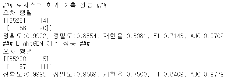
●로그변환을 이용해 Amount 피처 변환
def get_preprocessed_df(df=None):
    df_copy = df.copy()

    # Amount 피처를 로그변환
    amount_n = np.log1p(df_copy['Amount'])

    # 변환된 Amount 피처를 Amount_Scaled로 피처명 변경후 DataFrame 맨 앞 컬럼으로 추가
    df_copy.insert(0, 'Amount_Scaled', amount_n)

    # 기존 Time, Amount 피처 삭제
    df_copy.drop(['Time', 'Amount'], axis=1, inplace=True)

    return df_copy
●모델 학습/예측/평가
# Amount를 로그변환 후 모델 학습/예측/평가
X_train, X_test, y_train, y_test = get_train_test_dataset(card_df)

print('### 로지스틱 회귀 예측 성능 ###')
lr_clf = LogisticRegression(max_iter=1000)
get_model_train_eval(lr_clf, ftr_train=X_train, ftr_test=X_test, tgt_train=y_train, tgt_test=y_test)

print('### LightGBM 예측 성능 ###')
lgmb_clf = LGBMClassifier(n_estimators=1000, num_leaves=64, n_jobs=-1, boost_from_average=False)
get_model_train_eval(lgbm_clf, ftr_train=X_train, ftr_test=X_test, tgt_train=y_train, tgt_test=y_test)
4. 이상치 데이터 제거 후 모델 학습/예측/평가
●IQR을 이용해 이상치 데이터 제거
- 모든 피처들의 이상치를 검출하는 것은 시간이 많이 소모되며, 결정값과 상관성이 높지 않은 피처들의 경우는 이상치를 제거하더라도 크게 성능 향상에 기여하지 않기 때문에 매우 많은 피처가 있을 경우 이들 중 결정값과 가장 상관성이 높은 피처들을 위주로 이상치를 검출하는 것이 좋다.
import seaborn as sns

plt.figure(figsize=(9,9))
corr = card_df.corr() # DataFrame의 각 피처별로 상관관계를 구함
sns.heatmap(corr, cmap='RdBu') # 상관관계를 시본의 heatmap으로 시각화
상관관계 히트맵에서 Class와 음의 상관관계가 가장 높은 V14, V17 중 V14에 대해서만 이상치를 찾아서 제거해보자
# 이상치 데이터 검출
import numpy as np

def get_outlier(df=None, column=None, weight=1.5):
    quantile_25 = np.percentile(df[column].values, 25)
    quantile_75 = np.percentile(df[column].values, 75)

    iqr = quantile_75 - quantile_25
    iqr_weight = iqr * weight

    lowest = quantile_25 - iqr_weight
    highest = quantile_75 + iqr_weight

    # 최소와 최대 사이에 있지 않은 값은 이상치로 간주하고 인덱스 반환
    outlier_index = df[column][(df[column] < lowest) | (df[column] > highest)].index

    return outlier_index
outlier_index = get_outlier(df=card_df, column='V14', weight=1.5)
print('이상치 데이터 인덱스:', outlier_index)
print('이상치 데이터 개수:', len(outlier_index))
- 현재 creditcard 데이터는 전체 데이터를 기반으로 IQR을 설정하면 너무 많은 데이터가 이상치로 설정되서 삭제되는 범위가 너무 커짐
- 일반적으로 이상치가 이렇게 많다는 것은 말이 안된다고 판단, 그리고 이상치 제거는 가능한 최소치로 해줘야함
- 전체 데이터를 IQR로 하면 실제 사기 데이터에 잘 동작하는 데이터도 삭제 시켜버리고 있음
→creditcard 데이터(레이블이 불균형한 분포를 가진 불균형한 데이터)를 통해 생성한 모델은 실제값 0을 0으로 예측하는 것은 기본적으로 잘됨. 하지만 카드 사기 검출 모델에서 중요한 것은 실제 사기 즉 1을 1로 예측하는 것이 중요하므로 타겟값이 1인 데이터에 대해서 적절한 이상치를 제거하는 것이 필요함. 때문에 현재 데이터에서는 1의 데이터만 일정 수준에서 이상치를 제거해 주는게 좋음
# 타겟값이 1인 데이터에 대해서 이상치 데이터 검출
import numpy as np

def get_outlier(df=None, column=None, weight=1.5):
    fraud = df[df['Class']==1][column]

    quantile_25 = np.percentile(fraud, 25)
    quantile_75 = np.percentile(fraud, 75)

    iqr = quantile_75 - quantile_25
    iqr_weight = iqr * weight

    lowest = quantile_25 - iqr_weight
    highest = quantile_75 + iqr_weight

    # 최소와 최대 사이에 있지 않은 값은 이상치로 간주하고 인덱스 반환
    outlier_index = fraud[(fraud < lowest) | (fraud > highest)].index

    return outlier_index
outlier_index = get_outlier(df=card_df, column='V14', weight=1.5)
print('이상치 데이터 인덱스:', outlier_index)
# 이상치 데이터 제거
def get_preprocessed_df(df=None):
    df_copy = df.copy()

    # Amount 피처를 로그변환
    amount_n = np.log1p(df_copy['Amount'])

    # 변환된 Amount 피처를 Amount_Scaled로 피처명 변경후 DataFrame 맨 앞 컬럼으로 추가
    df_copy.insert(0, 'Amount_Scaled', amount_n)

    # 기존 Time, Amount 피처 삭제
    df_copy.drop(['Time', 'Amount'], axis=1, inplace=True)

    # 이상치 데이터 삭제하는 로직 추가
    outlier_index = get_outlier(df=df_copy, column='V14', weight=1.5)
    df_copy.drop(outlier_index, axis=0, inplace=True)

    return df_copy
●모델 학습/예측/평가
X_train, X_test, y_train, y_test = get_train_test_dataset(card_df)

print('### 로지스틱 회귀 예측 성능 ###')
lr_clf = LogisticRegression(max_iter=1000)
get_model_train_eval(lr_clf, ftr_train=X_train, ftr_test=X_test, tgt_train=y_train, tgt_test=y_test)

print('### LightGBM 예측 성능 ###')
lgbm_clf = LGBMClassifier(n_estimators=1000, num_leaves=64, n_jobs=-1, boost_from_average=False)
get_model_train_eval(lgbm_clf, ftr_train=X_train, ftr_test=X_test, tgt_train=y_train, tgt_test=y_test)
5. SMOTE 오버 샘플링 적용 후 모델 학습/예측/평가
재샘플링, 즉 오버 샘플링 및 언더 샘플링을 적용시 올바른 평가를 위해 반드시 학습 데이터 세트에만 적용해야함
●SMOTE 오버 샘플링 적용
from imblearn.over_sampling import SMOTE

smote = SMOTE(random_state=0)
X_train_over, y_train_over = smote.fit_resample(X_train, y_train) # X_train, y_train은 4번 과정까지 전처리 된 후 split된 데이터

# 데이터 확인
print('SMOTE 적용 전 학습용 데이터 세트:', X_train.shape, y_train.shape)
print('SMOTE 적용 후 학습용 데이터 세트:', X_train_over.shape, y_train_over.shape)
print('SMOTE 적용 후 레이블 값 분포')
print(pd.Series(y_train_over).value_counts())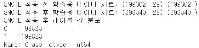
●모델 학습/예측/평가
print('### 로지스틱 회귀 예측 성능 ###')
lr_clf = LogisticRegression(max_iter=1000)
get_model_train_eval(lr_clf, ftr_train=X_train_over, ftr_test=X_test, tgt_train=y_train_over, tgt_test=y_test)

print('### LightGBM 예측 성능 ###')
lgbm_clf = LGBMClassifier(n_estimators=1000, num_leaves=64, n_jobs=-1, boost_from_average=False)
get_model_train_eval(lgbm_clf, ftr_train=X_train_over, ftr_test=X_test, tgt_train=y_train_over, tgt_test=y_test)
로지스틱 회귀는 SMOTE 적용 후 재현율이 92.47%로 크게 증가했지만 정밀도가 5.4%로 급격하게 감소했음. 재현율이 높더라도 이 정도로 저조한 정밀도로는 현실 업무에 적용할 수 없음.
로지스틱 회귀 모델에 어떠한 문제가 발생하고 있는지 분류 결정 임계값(threshold)에 따른 정밀도와 재현율 곡선을 통해 알아보자.
precisions, recalls, thresholds = precision_recall_curve(y_test, lr_clf.predict_proba(X_test)[:, 1])

# x축을 threshold값, y축은 정밀도, 재현율 값으로 각각 plot 수행, 정밀도는 점선으로 표시
plt.figure(figsize=(8,6))
threshold_boundary = thresholds.shape[0]
plt.plot(thresholds, precisions[0:threshold_boundary], linestyle='--', label='precision')
plt.plot(thresholds, recalls[0:threshold_boundary], label='recall')

# threshold 값 x축의 scale을 0.1 단위로 변경
start, end = plt.xlim()
plt.xticks(np.round(np.arange(start, end, 0.1), 2))

# x, y축 labe과 legend, grid 설정
plt.xlabel('Threshold value')
plt.ylabel('Precision and Recall value')
plt.legend()
plt.grid()
plt.show()
(번외로, LightGBM 모델도 precision_recall_curve를 그리려면 다음과 같이 함수를 만드는 것이 편리)
from sklearn.metrics import precision_recall_curve

def precision_recall_curve_plot(y_test, pred_proba_c1):
    # threshold ndarray와 이 threshold에 따른 정밀도, 재현율 ndarray 추출
    precisions, recalls, thresholds = precision_recall_curve(y_test, pred_proba_c1)

    # x축을 threshold값, y축은 정밀도, 재현율 값으로 각각 plot 수행, 정밀도는 점선으로 표시
    plt.figure(figsize=(8,6))
    threshold_boundary = thresholds.shape[0]
    plt.plot(thresholds, precisions[0:threshold_boundary], linestyle='--', label='precision')
    plt.plot(thresholds, recalls[0:threshold_boundary], label='recall')

    # threshold 값 x축의 scale을 0.1 단위로 변경
    start, end = plt.xlim()
    plt.xticks(np.round(np.arange(start, end, 0.1), 2))

    # x, y축 labe과 legend, grid 설정
    plt.xlabel('Threshold value')
    plt.ylabel('Precision and Recall value')
    plt.legend()
    plt.grid()
    plt.show()
precision_recall_curve_plot(y_test, lr_clf.predict_proba(X_test)[:, 1])precision_recall_curve_plot(y_test, lgbm_clf.predict_proba(X_test)[:, 1])threshold가 0.99 이하에서는 재현율이 매우 좋고, 정밀도가 극단적으로 낮다가 0.99 이상에서는 반대로 재현율이 대폭 떨어지고 정밀도가 높아짐. threshold를 조정하더라도 threshold의 민감도가 너무 심해 올바른 재현율/정밀도 성능을 얻을 수 없으므로 로지스틱 회귀 모델의 경우 SMOTE 적용 후 올바른 예측 모델이 생성되지 못했음.
LightGBM의 모델 성능 결과를 보면, 재현율은 증가했지만 정밀도가 감소했음을 알 수 있음. 이처럼 SMOTE를 적용하면 재현율은 높아지나, 정밀도는 낮아지는 것이 일반적임. 때문에 정밀도 지표보다 재현율 지표를 높이는 것이 중요한 업무에서SMOTE를 사용하면 좋음!
'파이썬 머신러닝 완벽가이드 > [4장] 분류' 카테고리의 다른 글
| Feature Selection의 이해(1) (0) | 2023.03.03 |
|---|---|
| 스태킹 앙상블 (0) | 2023.02.27 |
| 캐글 신용카드 사기 검출(log 변환, 이상치 제거, SMOTE 오버샘플링 기초지식) (0) | 2023.02.24 |
| 캐글 산탄데르 고객 만족 예측 (0) | 2023.02.23 |
| 베이지안 최적화 기반의 HyperOpt를 이용한 하이퍼 파라미터 튜닝(2) (0) | 2023.02.22 |