차원의 저주 문제(특징 선택)
차원의 저주란?
차원(특징 수)이 증가함에 따라 필요한 데이터의 양과 시간 복잡도가 기하급수적으로 증가하는 문제를 의미한다.
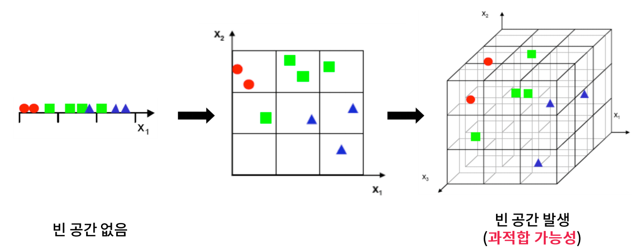
차원이 증가함에 따라서 각 공간에 들어가는 샘플이 적어질 수 밖에 없기 때문에 정확한 판단을 위해서는 샘플이 더 많아질 수 밖에 없다. 그리고 샘플이 더 많게 하기 위해서는 데이터를 더 수집해야 하기 때문에 쉬운 문제가 아니다. 그래서 샘플이 부족하기 때문에 과적합으로 이어질 것이다. 특징이 범주형인 경우에 비해서 연속형인 경우 특징이 늘면 공간이 더 세분화되고 더 늘어날 수 있어서 단순히 특징이 많고 적고도 고려해야하고 특징의 종류도 고려해야한다.
●차원을 줄여야 하는 이유(특징 개수를 줄여야 하는 이유)
1. 차원이 증가함에 따라 모델 학습 시간이 정비례하게 증가한다.
2. 차원이 증가하면 각 결정 공간에 포함되는 샘플 수가 적어져, 과적합으로 이어져 성능 저하가 발생할 수 있다.

특징이 너무 적으면 과소적합이 일어날 수 있고, 특징이 늘어날수록 모델 성능이 올라가다가 어느 순간에 떨어질 것이다. 이 떨어지는 구간이 과적합이 발생한 구간이다.
차원의 저주 해결방법: 특징 선택
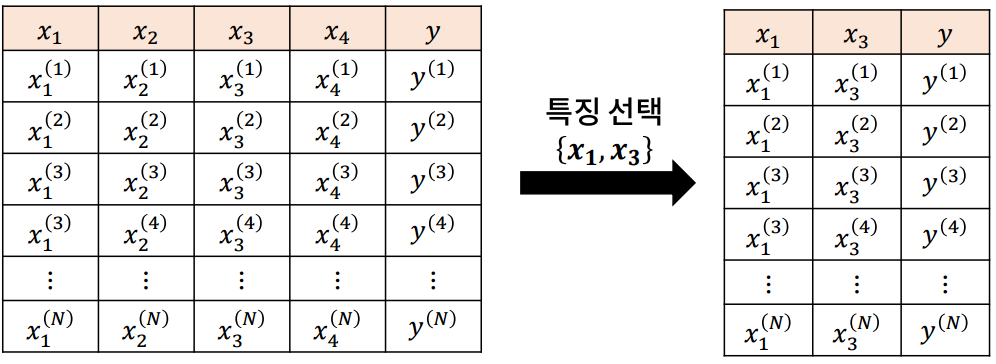
특징 선택은 분류 및 예측에 효과적인 특징만 선택하여 차원을 축소하는 방법이다. 구체적으로 설명하자면 n개의 특징으로 구성된 특징 집합 {x1, x2, ..., xn}에서 m < n개의 특징을 선택하여, 새로운 특징 집합 {x'1, x'2, ..., x'm} ⊂ {x1, x2, ..., xn}을 구성하는 방법이다.
특징 선택을 할 때 많이 하는 오해가 있는데 특징 선택을 할 때는 특징이 많은 데이터에만 정의해야 한다고 오해하는 것이다. 즉, 특징 선택은 특징이 많은 데이터에만 적용해야 하는 것은 아니다. 왜냐하면 특징이 적더라도 특징 선택을 했을 때 모델의 성능이 좋아지는 경우가 존재하기 때문이다.
## 코드 실습 ##
import os
os.chdir(r"C:\Users\82102\Desktop\study\데이터전처리\머신러닝 모델의 성능 향상을 위한 전처리\5. 머신러닝 모델의 성능 향상을 위한 전처리\데이터")

import pandas as pd
df = pd.read_csv("appendicitis.csv")
df.head()
# 특징과 라벨 분리
X = df.drop('Class', axis=1)
Y = df['Class']
# 학습 데이터와 평가 데이터 분리
from sklearn.model_selection import train_test_split
x_train, x_test, y_train, y_test = train_test_split(X, Y)# 특징에 따른 SVM 모델 테스트 함수 작성
from sklearn.svm import SVC
from sklearn.metrics import f1_score
def feature_test(x_train, x_test, y_train, y_test, features):
s_x_train = x_train[features]
s_x_test = x_test[features]
model = SVC().fit(s_x_train, y_train)
pred_y = model.predict(s_x_test)
return f1_score(y_test, pred_y)
base_score = feature_test(x_train, x_test, y_train, y_test, x_train.columns) # 모든 특징을 썼을 때의 점수
print(base_score)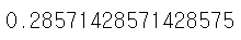
import itertools
c_list = list(range(1, len(x_train.columns))) # base_score: 모든 특징을 사용한 경우는 제외
outperform_ratio_list = []
best_score = 0

for c in c_list: # c는 선택한 특징 개수
    print(c)
    c_num = 0 # 특징을 c개 뽑았을 때, 모든 특징을 썼을 때보다 성능이 좋은 경우
    c_dem = 0 # 특징을 c개 뽑는 경우의 수

    # itertools.combinations(p,r): 이터레이터 객체 p에서 크기 r의 가능한 모든 조합을 갖는 이터레이터를 생성
    for features in itertools.combinations(x_train.columns, c):
        score = feature_test(x_train, x_test, y_train, y_test, list(features)) # itertools는 tuple 형태로 값을 반환해서 형변환을 해줌
        if score > best_score:
            best_score = score
            best_feature = list(features)

        if score > base_score:
            c_num += 1

        c_dem += 1

    outperform_ratio_list.append(c_num / c_dem)
    # 예를 들어, 특징 개수를 한 개 뽑는다면 6개의 combination이 있는데
    # 6개의 combination의 score값이 base_score보다 큰 경우 c_num을 1씩 더해서 업데이트
    # c_dem은 combination의 값과 동일: 특징 개수를 한 개 뽑는다면 경우의 수가 6개
%matplotlib inline
from matplotlib import pyplot as plt
plt.bar(c_list, outperform_ratio_list)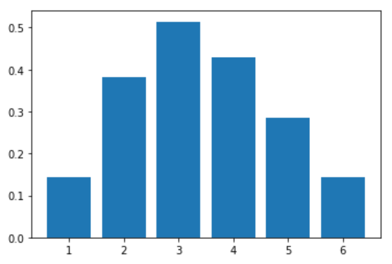
best_feature, best_score
위의 코드는 특징이 7개인 데이터에 대해, 모든 특징 집합을 비교해 본 결과이다.
모든 특징을 사용했을 때의 성능 f1-score는 0.2857이지만 특징을 [At1, At4] 두 개만 쓰는 경우 0.7499로 가장 좋은 성능을 확인 할 수 있다.
이런 주먹구구식 특징 선택은 선택 가능한 모든 특징 집합을 비교/평가하여 가장 좋은 특징 집합을 선택할 수 있지만 특징 개수가 많아지면 현실적으로 불가능하다. 즉, 최적의 결과를 보장할 수 있지만 최적의 결과를 얻기까지 시간이 너무 오래걸린다.
→특징 개수가 n개라면, 2^n-1번의 모형 학습이 필요하므로, 현실적으로 적용 불가능하다. 1초에 1억 번의 모형을 학습할 수 있는 슈퍼 컴퓨터가, 1000개의 특징이 있는 데이터에 대해, 이 방법을 적용하여 가장 좋은 특징 집합을 선택하는데 소요되는 시간은 400조년이다.
이런 문제점을 해결하기 위한 방법을 아래에서 볼 것이다.
클래스 관련성 기반의 특징 선택
특징과 라벨이 얼마나 관련이 있는지를 나타내는 클래스 관련성이 높은 특징을 우선 선택하는 방법이다.

클래스 관련성은 한 특징이 클래스를 얼마나 잘 설명하는지를 나타내는 척도로 특징과 라벨 간 독립성을 나타내는 통계량상관계수, 카이제곱 통계량, 상호정보량 등을 사용하여 측정한다.(서로 독립적이면 특징은 라벨을 예측하는데 도움이 안될 것이고 서로 종속적이면 특징은 라벨을 예측하는데 도움이 될 것이다.)
즉, 클래스 관련성이 높은 특징은 분류 및 예측에 도움이 되는 특징이며, 그렇지 않은 특징은 도움이 되지 않는 특징이다.
예를 들어, 특징이 범주형이고 라벨도 범주형인 상황(범주형 특징-분류)
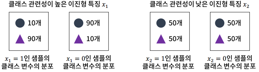
x1이 1이면 y는 90% 세모라고 분류를 해 줄 것이고, x1이 0이면 y는 90% 동그라미라고 분류를 해 줄 것이다. 원래 데이터의 분포가 5대5였는데, x1이 1이면 y가 세모일 확률이 높아지고, x1이 0이면 y가 동그라미일 확률이 높아지는 것을 보고 x1과 y가 크게 관련이 있다는 것을 알 수 있다.
반대로 x2를 보면 x2가 1이거나 0이거나 관계없이 둘 다 5대5로 똑같다. 다시 말해 원래 데이터의 분포도 5대5(동그라미 100개, 세모 100개)였는데, x2가 주어지던 안주어지던 상관이 없다. 그러면 x2를 알고 있으나 모르고 있으나 크게 도움이 안되니까 x2는 라벨을 분류하는데 도움이 안되는 특징이다.
클래스 관련성 척도 중 대표적으로 많이 쓰는 F-통계량을 살펴보겠다.
F-통계량은 일원분산분석(ANOVA)에서 사용하는 통계량으로, 집단 간 평균 차이가 있는지를 측정하기 위한 통계량이다.

x1의 값에 따라 y 분류가 어느정도 가능하지만, x2는 그렇지 않다.
★클래스 관련성 척도 분류

(범주형 변수를 더미화 했기 때문에 특징 유형이 이진형이다.)
●관련 함수: sklearn.feature_selection.SelectKBest
-주요 입력
▷scoring_func: 클래스 관련성 측정 함수(예: chi2, mutual_info_classif 등)
▷k: 선택하는 특징 개수
-주요 메서드
▷.fit, .transform, .fit_transform: 특징을 선택하는데 사용하는 메서드
▷.get_support(): 선택된 특징의 인덱스를 반환
-주요 속성
▷scores_: scoring_func으로 측정한 특징별 점수
▷pvalues_: scoring_func으로 측정한 특징별 p-value(1에 가까울수록 독립적이며, 0에 가까울수록 관련성이 높음→작을수록 좋은 특징)
→score자체를 보는 경우는 드물고 pvalue를 바탕으로 독립적인지 아닌지를 측정한다. pvalue를 보는 경우는 k값을 따로 설정하지 않고 pvalue가 얼마 미만인 경우만 고르는 경우라던가 특징 유형이 다른 경우에 관련 함수가 달라지기 때문에 그 때 통계량을 비교하기 어려우니 pvalue로 비교한다.
특징 유형이 다른 경우 pvalue로 비교하는 방법 말고 다른 방법은 상호 정보량을 이용한다.
## 코드 실습 ##
●모든 특징 유형이 같은 경우의 특징 선택
import os
os.chdir(r"C:\Users\82102\Desktop\study\데이터전처리\머신러닝 모델의 성능 향상을 위한 전처리\5. 머신러닝 모델의 성능 향상을 위한 전처리\데이터")

import pandas as pd
df = pd.read_csv("Sonar_Mines_Rocks.csv")
df.head()
# 특징과 라벨 분리
X = df.drop('Y', axis=1)
Y = df['Y']
# 모든 특징 연속형
for i in X.columns:
print(i, len(df[i].unique()))Band1 65
Band2 83
Band3 90
Band4 92
Band5 112
Band6 134
Band7 133
Band8 139
Band9 154
Band10 162
Band11 164
Band12 168
Band13 168
Band14 169
Band15 176
Band16 179
Band17 177
Band18 175
Band19 173
Band20 179
Band21 187
Band22 183
Band23 173
Band24 175
Band25 181
Band26 171
Band27 173
Band28 168
Band29 179
Band30 182
Band31 190
Band32 184
Band33 185
Band34 184
Band35 188
Band36 188
Band37 180
Band38 172
Band39 166
Band40 183
Band41 175
Band42 172
Band43 173
Band44 154
Band45 162
Band46 151
Band47 147
Band48 131
Band49 98
Band50 50
Band51 45
Band52 39
Band53 32
Band54 31
Band55 29
Band56 27
Band57 27
Band58 28
Band59 29
Band60 24# 학습 데이터와 평가 데이터 분리
from sklearn.model_selection import train_test_split
x_train, x_test, y_train, y_test = train_test_split(X, Y)# 라벨이 문자이니 변환
y_train.replace({"M":-1, "R":1}, inplace=True)
y_test.replace({"M":-1, "R":1}, inplace=True)x_train.shape
# 특징 선택 전 성능 확인(특징이 연속형이고 분류 문제)
from sklearn.neighbors import KNeighborsClassifier as KNN
from sklearn.metrics import f1_score

model = KNN().fit(x_train, y_train)
pred_y = model.predict(x_test)
print(f1_score(y_test, pred_y))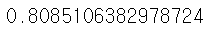
# 특징 선택 수행
from sklearn.feature_selection import *

selector = SelectKBest(f_classif, k = 30)
selector.fit(x_train, y_train)
selected_features = x_train.columns[selector.get_support()]

s_x_train = pd.DataFrame(selector.transform(x_train), columns = selected_features)
s_x_test = pd.DataFrame(selector.transform(x_test), columns = selected_features)
# transform을 해도되지만 get_support()를 통해 추출한 특징을 바로 슬라이싱 가능
# s_x_train = x_train[selected_features], s_x_test = x_test[selected_features]
# 특징 선택 후 성능 확인
model = KNN().fit(s_x_train, y_train)
pred_y = model.predict(s_x_test)
print(f1_score(y_test, pred_y))
# 특징 개수 튜닝
best_score = 0

for k in range(5, 50, 5):
    selector = SelectKBest(f_classif, k = k)
    selector.fit(x_train, y_train)
    selected_features = x_train.columns[selector.get_support()]

    s_x_train = pd.DataFrame(selector.transform(x_train), columns = selected_features)
    s_x_test = pd.DataFrame(selector.transform(x_test), columns = selected_features)

    model = KNN().fit(s_x_train, y_train)
    pred_y = model.predict(s_x_test)
    score = f1_score(y_test, pred_y)
    if score > best_score:
        best_score = score
        best_k = k

print(best_score, best_k)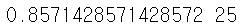
●특징 유형이 다른 경우의 특징 선택
import os
os.chdir(r"C:\Users\82102\Desktop\study\데이터전처리\머신러닝 모델의 성능 향상을 위한 전처리\5. 머신러닝 모델의 성능 향상을 위한 전처리\데이터")

import pandas as pd
df = pd.read_csv("australian.csv")
df.head()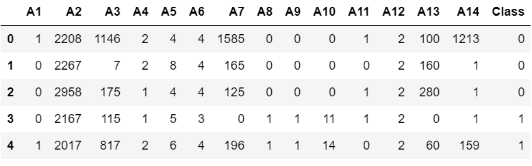
# 특징과 라벨 분리
X = df.drop('Class', axis=1)
Y = df['Class']
# 학습 데이터와 평가 데이터 분리
from sklearn.model_selection import train_test_split
x_train, x_test, y_train, y_test = train_test_split(X, Y)x_train.shape
# 특징 선택 전 성능 확인
from sklearn.neighbors import KNeighborsClassifier as KNN
from sklearn.metrics import f1_score

model = KNN().fit(x_train, y_train)
pred_y = model.predict(x_test)
print(f1_score(y_test, pred_y))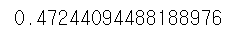
데이터 설명서를 보면 연속형 특징과 범주형 특징이 섞여있고 분류 문제이다.
# 유니크한 값의 개수를 바탕으로 연속형과 범주형 변수 구분
# type과 상태공간을 확인해야하지만 3을 기준으로 연속형인지 범주형인지 구분 할 수 있다고 가정
continuous_cols = [col for col in x_train.columns if len(x_train[col].unique()) > 3]
category_cols = [col for col in x_train.columns if len(x_train[col].unique()) <= 3]
이 데이터는 분류 문제이기 때문에 범주형 특징에 대해서는 카이제곱 통계량이 적절하고, 연속형 특징에 대해서는 F-통계량이 적절하다. 카이제곱 통계량과 F-통계량을 통계량 기준으로 구분하기 쉽지 않기 때문에 pvalue만 계산해서 pvalue가 작은 것 순서대로 선택을 할 것이다.
# 연속형 변수에 대해서는 f_classif, 범주형 변수에 대해서는 chi2를 적용
from sklearn.feature_selection import *

# scoring_func(x, y)의 결과 -> (statistics, p-value)
continuous_cols_pvals = f_classif(x_train[continuous_cols], y_train)[1]
category_cols_pvals = chi2(x_train[category_cols], y_train)[1]
print(continuous_cols_pvals)
print('\n')
print(category_cols_pvals)
# 각각을 Series로 변환(value: pvalue, index: column name)
continuous_pvals_s = pd.Series(continuous_cols_pvals, index = continuous_cols)
category_pvals_s = pd.Series(category_cols_pvals, index = category_cols)
continuous_pvals_s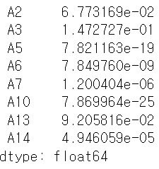
category_pvals_s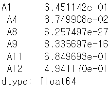
# 두 Series를 합친 뒤, 오름차순으로 정렬
pvals = pd.concat([continuous_pvals_s, category_pvals_s])
pvals.sort_values(ascending=True, inplace=True)
pvals
# pvalue가 작은 것 순서대로 선택(앞에 나오는 특징부터 좋은 특징)
# 특징 선택
k = 10

s_x_train = x_train[pvals.iloc[:k].index]
s_x_test = x_test[pvals.iloc[:k].index]
# 특징 선택 후 성능 확인
model = KNN().fit(s_x_train, y_train)
pred_y = model.predict(s_x_test)
print(f1_score(y_test, pred_y))
# 특징 개수 튜닝
best_score = 0

for k in range(1, 14, 1):
    s_x_train = x_train[pvals.iloc[:k].index]
    s_x_test = x_test[pvals.iloc[:k].index]

    model = KNN().fit(s_x_train, y_train)
    pred_y = model.predict(s_x_test)
    score = f1_score(y_test, pred_y)
    if score > best_score:
        best_score = score
        best_k = k

print(best_score, best_k)
연속형 변수와 범주형 변수가 섞여있을 때 위의 과정은 좀 귀찮고 편하게 하고 싶으면 상호 정보량을 이용한다.
# 상호 정보량을 이용한 특징 선택 수행
selector = SelectKBest(mutual_info_classif, k = 10)
selector.fit(x_train, y_train)
selected_features = x_train.columns[selector.get_support()]

s_x_train = pd.DataFrame(selector.transform(x_train), columns = selected_features)
s_x_test = pd.DataFrame(selector.transform(x_test), columns = selected_features)
# 상호 정보량을 이용한 특징 선택 후 성능 확인
model = KNN().fit(s_x_train, y_train)
pred_y = model.predict(s_x_test)
print(f1_score(y_test, pred_y))
# 특징 개수 튜닝
best_score = 0

for k in range(1, 14, 1):
    selector = SelectKBest(mutual_info_classif, k = k)
    selector.fit(x_train, y_train)
    selected_features = x_train.columns[selector.get_support()]

    s_x_train = pd.DataFrame(selector.transform(x_train), columns = selected_features)
    s_x_test = pd.DataFrame(selector.transform(x_test), columns = selected_features)

    model = KNN().fit(s_x_train, y_train)
    pred_y = model.predict(s_x_test)
    score = f1_score(y_test, pred_y)
    if score > best_score:
        best_score = score
        best_k = k

print(best_score, best_k)
특징 선택 — 데이터 사이언스 스쿨
.ipynb .pdf to have style consistency -->
datascienceschool.net
의사결정나무, 랜덤포레스트 등 모델 기반 특징을 선택하는 방법도 있다는 것을 알게됨